My open-source NEPTUNE (N-body Exoplanet Prediction Using TTV for Unseen Exoplanets) pipeline is an attempt to detect and characterise unseen exoplanets, by analysing their gravitational perturbations in the transit timings of the exoplanets we can observe. This post details how NEPTUNE was built, how it works, how it was validated against known systems, and what the expansion steps are, including extending it to long-period planets for which we have only been able to capture a single transit.
NEPTUNE: In brief
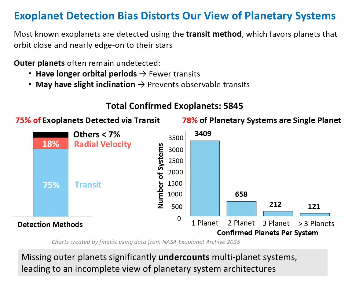
Transit surveys are biased towards discovering planets that are easier to detect: short-period planets with nearly edge-on orbits that produce the most frequent and most observable dips in transit light curves. Multi-planet systems whose outer companions are long-period or inclined produce less frequent dips. They are also more likely to be non-transiting from our line of sight, and are missed as a matter of geometry rather than rarity. NEPTUNE addresses that gap by analysing the variations in transit-timings of the planet we can see in order to possibly detect and characterise the one we cannot.
The core of NEPTUNE is 80,000 N-body simulations spanning eleven stellar and planetary parameters, capturing the gravitational interaction across two very different timescales: long-period resonant signals, and the short-period synodic signal set by planetary conjunctions. Those simulations train a Random Forest whose predictions become informed priors for Bayesian MCMC (Markov Chain Monte Carlo), reducing the compute needed for convergence to a solution by roughly a factor of eight. They also show why analysing multiple periods at once matters. The resonant signal depends on both the unseen planet's mass and its eccentricity while the synodic signal is eccentricity-independent. Analysing both signals together breaks the mass-eccentricity degeneracy and returns a single solution with quantified uncertainties. The physics of that degeneracy-breaking is well established (Deck & Agol 2015) but what is new about NEPTUNE is the end-to-end pipeline pivoted on simulations and priors that applies it automatically, and can be run on computational resources available to citizen scientists.
When run on Kepler-46b transit-timing data, NEPTUNE recovers the unseen Kepler-46c at a period of 57 days, an eccentricity of 0.014 and a mass of 110 Earth masses, consistent with published analyses of the system. Applied to Kepler-1710b, an understudied system that exhibits transit-timing variations, it produced a solution pointing to a possible companion of roughly 27.5 Earth masses. Integrating NEPTUNE with data from NASA's TESS mission and ESA's ExoClock initiative would extend its reach.
The Challenge: A biased view of planetary systems
Most of the roughly 5,845 confirmed exoplanets were found by the transit method, which only works for planets on short, nearly edge-on orbits. Outer planets have longer periods and, as they are slightly inclined, they often never transit from our line of sight. So about 78% of known systems appear to be single-planet. That is a methodological bias, not reality: we are missing the outer planets, which distorts our picture of how planetary systems are built.
How transit-timing variations reveal hidden planets
In a single-planet system, transits arrive like clockwork. But if an unseen companion is added, its gravity tugs the transiting planet, making each transit arrive slightly early or late. Plotted over time, those shifts trace a periodic observed-minus-calculated (O-C) curve. The same principle revealed planet Neptune itself, from the timing anomalies of Uranus. Analysing these curves backwards can recover probable combinations of mass and period for the unseen, non-transiting planet.

Why TTV analysis needs to be automated and accelerated
In spite of the uniqueness of the TTV method to detect unseen planets, only about 36 exoplanets have been confirmed through TTVs. But there is potential for more. Archived Kepler data alone shows roughly 260 strong signals still undecoded (Holczer et al. 2016). The analysis is difficult for two reasons: it needs long baselines (possibly combining Kepler and TESS epochs, and data from ground-based surveys), and it is degenerate: as Lithwick, Xie & Wu (2012) showed analytically, a high-mass, low-eccentricity planet and a low-mass, high-eccentricity one can produce almost the same O-C curve. NEPTUNE can analyse the available data and attempt to break that degeneracy automatically.

NEPTUNE Methodology: Built on open science, open source, open data
Every input used by NEPTUNE is open data. These include transit catalogues from Kepler and TESS, ephemerides from the NASA Exoplanet Archive, radial-velocity data from HARPS, and observations from shared robotic telescopes (Alnitak in Spain, Burke-Gaffney in Canada). Every tool is open-source: REBOUND (Rein & Liu 2012) for the N-body integration with the IAS15 integrator (Rein & Spiegel 2015) adapted to TTV, SciPy/Astropy, scikit-learn for the machine learning, and emcee (Foreman-Mackey et al. 2013) for the Bayesian inference. Anyone can reproduce or modify the code: it is on GitHub at github.com/Spacegirl123/ExoplanetTTV.

Step 1: 80,000 N-body simulations
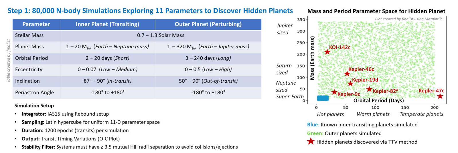
To learn what TTV signals look like, I simulated 80,000 two-planet systems with the REBOUND IAS15 integrator (Rein & Liu 2012; Rein & Spiegel 2015), spanning 11 parameters: stellar mass, both planets' masses, orbital periods, eccentricities, inclinations, and periastron angles - sampled by Latin hypercube for even coverage. Each system ran 1,200 transit epochs, and I kept only dynamically stable configurations (companions separated by at least 3.5 mutual Hill radii). The result is a library of realistic O-C curves with known answers.

Reading the O-C curve: Three signals in one
A real O-C curve is not one clean sinusoid but a sum of signals on different timescales: a short synodic signal from planetary conjunctions, a dominant resonance-driven signal on months-to-years periods, and a slow apsidal-precession drift. Separating them in a periodogram is what makes the individual pieces of physical information recoverable. As shown next, the synodic signal is the key to breaking the mass-eccentricity degeneracy.

Steps 2 and 3: Extracting features, machine learning, and learning priors
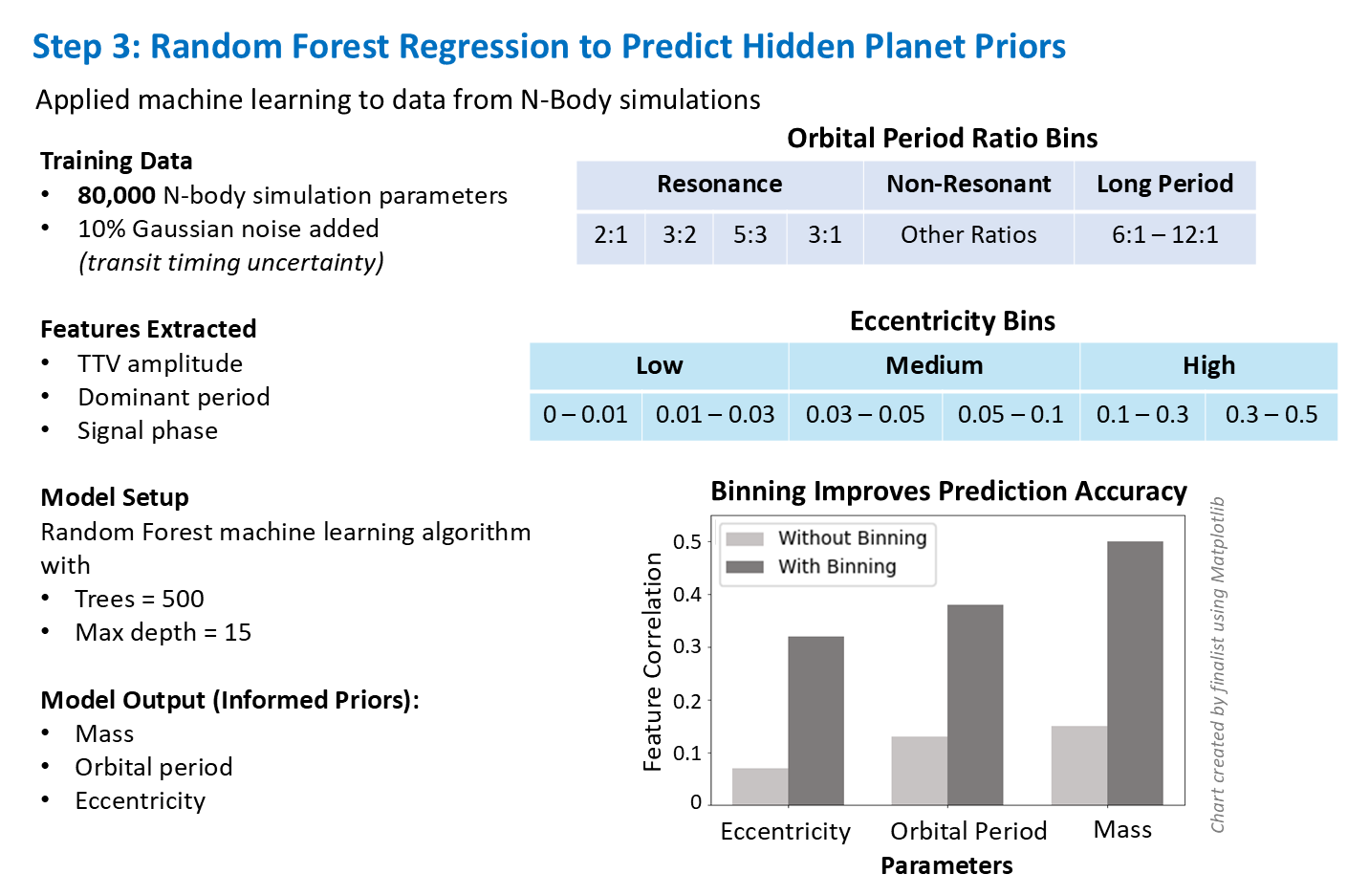
From each simulated curve I extract several features: the dominant period (via Lomb-Scargle; VanderPlas 2018), a secondary period, the amplitude, and a false-alarm probability, keeping only signals with FAP < 0.01. A Random Forest (500 trees, max depth 15), trained on the 80,000 simulations with 10% added noise, then learns to predict a hidden planet's mass, orbital period, and eccentricity directly from those features. Binning the training set by orbital-period ratio and eccentricity measurably sharpens the predictions.
Step 4: Bayesian inference recovers the parameters
The machine-learning predictions become informed starting points for a Markov Chain Monte Carlo fit (emcee; 100 walkers, 10,000 steps) that samples the full posterior with proper uncertainties. Convergence is verified with trace plots, autocorrelation, and the Gelman-Rubin statistic (trusted only when R < 1.1). A converged chain yields clean, stable corner plots while a non-converged one is visibly unstable.

Result 1: Mapping the TTV signals with varying mean-motion resonances, perturbing masses and eccentricities
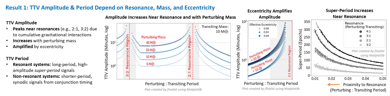
The first result maps how the TTV signal behaves. TTV amplitude peaks sharply near mean-motion resonances (2:1, 3:2), increases with the perturbing planet's mass, and is amplified by eccentricity. Resonant systems produce long-period, high-amplitude super-period signals; non-resonant ones give shorter synodic signals tied to conjunctions. Knowing these dependencies is what lets NEPTUNE invert a curve into physical parameters.
Result 2: Recovering synodic signal to break the mass-eccentricity degeneracy
The “chopping” route to a perturber’s mass was derived by Deck & Agol (2015), building on the degeneracy identified by Lithwick, Xie & Wu (2012). NEPTUNE adds an automated pipeline that applies it without hand-tuning. The synodic signal has a period set by orbital geometry (independent of mass and eccentricity) but an amplitude that grows with perturbing mass. Thus it carries mass information about the perturbing planet that the dominant signal alone cannot. Applying NEPTUNE, I was able to pick the correct solution for unseen Kepler-46c where a naive fit is degenerate with multiple solutions. The predicted synodic peak matches the observed one for the right parameters and misses it for the wrong ones.

Result 3: Recovering a known hidden planet (Kepler-46c) in multiplanetary system
Given the 30 mid-transit times of Kepler-46b, NEPTUNE detected a strong TTV signal (period 191.5 ± 0.5 d, amplitude 59.1 ± 1.8 min, FAP ~10^-7). Feeding the Random-Forest priors into MCMC, it then recovered the unseen Kepler-46c at a period of 57.16 ± 0.40 d and a mass of 110 ± 2 Earth masses (statistical). The published values are 57.011 (+0.051/-0.061) d and 119.5 (+6.7/-6.0) Earth masses. Kepler-46c was originally detected and characterised this way by Nesvorný et al. (2012). Recovering the published answer from timing alone demonstrates that the method works.

Result 4: Deriving TTV signal solution in a single-planet system (Kepler-1710)
Applied to Kepler-1710, catalogued as a single-planet system, NEPTUNE reprocessed 70+ transits (via EXOTIC; Zellem et al. 2020) and found a significant timing signal (dominant O-C period 259.4 ± 0.3 d, amplitude 37.6 ± 1.5 min, FAP ~10^-11). The best fit would be an unseen, Neptune-mass companion of about 27.5 Earth masses near a 3:2 resonance, which also satisfies the system's radial-velocity constraints (< 1.23 Jupiter masses at 10 AU). This is a possible solution to the TTV signal, not a confirmed detection. It points to the need for further analysis, and is exactly the kind of solution the method is designed to surface.

Why informed priors matter: about 8x faster
The machine-learning step makes the method scalable. With uniform priors, the MCMC walkers wander through unlikely parameter space and take ~2,000 steps (weeks) to converge. With the Random-Forest-informed priors, they start in the right region and converge in ~250 steps (days), roughly 8x faster, which is the difference between analysing one system and analysing a survey.

Characterising the hidden planets
Once masses and orbits are recovered, NEPTUNE can characterise the planets: classifying them as rocky (< 10 Earth masses), Neptune-like (10-100), or gas giants (> 100), and estimating equilibrium temperature and habitable-zone status. Kepler-46c comes out as a ~110 Earth-mass gas giant (0.28 AU, 472 K); the possible Kepler-1710 candidate as a ~27.5 Earth-mass Neptune-like world (0.15 AU, 658 K). Both would be uninhabitable.

Determining planetary migration and architecture
The recovered parameters can also provide some information about the evolution of multiplanetary systems. Planet pairs often sit just wide of exact resonance (Kepler-25 b,c at a 2.04 period ratio; Kepler-46 b,c at 1.70), a signature of migration and tidal evolution. Following the architecture classification of Howe et al. (2025), mapping masses against periods distinguishes uniform peas-in-a-pod systems from hot-Jupiter systems. Thus a timing measurement becomes a window on how the system formed.


Errors and limitations
Mid-transit uncertainties from the light curves are propagated through the algorithm, the parameter estimates carry 1-sigma credible intervals, and competing models are ranked by sum of squared errors (lower is better). Because the N-body integrations ran on a home computer, they were limited to 200 steps per orbit.

What is next: Long-period planets with only single-transit information
The hardest planets to study are the ones that cross their star only once in the whole dataset. A planet on a wide, long-period orbit may transit a single time across the entire Kepler or TESS baseline, enough to know that something passed in front of the star, but not enough to establish a period, and so not enough to justify scheduling a follow-up. KOI 4307 and KOI 1271 are two such cases, and there are many more sitting unexamined for the same reason. Feedback at NASA's KOINet (Kepler Object of Interest Network) research meetings pointed to exactly this application: constraining long-period companions in systems such as KOI 4307.02, where only a single transit exists and the prospect of further data is remote.
The forward model behind NEPTUNE applies directly to this problem. A single transit fixes one epoch and a rough size, but leaves the period almost entirely open; every candidate period implies a different perturbation on any other transiting planet in the system. That turns an unconstrained problem into a constrained one: the timing residuals of a companion that transits repeatedly can rule out large parts of the period range that the single transit alone would allow. I am extending the simulation library in that direction, sampling the long-period, high-eccentricity configurations a lone transit is consistent with and testing which of them the existing timing data already excludes.
Conclusions
NEPTUNE integrates machine learning and Bayesian inference to detect and characterise hidden exoplanets rapidly, about 8x faster than uniform-prior fitting. It resolves the mass-eccentricity degeneracy through multi-period (synodic) fitting, and validates against well-studied systems with full uncertainty quantification. NEPTUNE is scalable. It already flagged a possible candidate companion in Kepler-1710 with probable mass and period solutions, and the open-source release lets others apply it to the hundreds of understudied TTV systems.
Open science, impact, and what is next
The code and training modules are open-source at github.com/Spacegirl123/ExoplanetTTV, so citizen scientists can help analyse the backlog of TTV systems. NEPTUNE received the Third Grand Award in Physics and Astronomy at the 2025 Regeneron International Science and Engineering Fair.

The Kepler-46c and Kepler-1710b results here use archival transit times from NASA's Kepler and TESS missions (MAST archive and the NASA Exoplanet Archive), not new telescope observations.
References
- Deck, K. M. & Agol, E. (2015). Measurement of planet masses with transit timing variations due to synodic "chopping" effects. ApJ, 802(2), 116. https://doi.org/10.1088/0004-637X/802/2/116
- Foreman-Mackey, D., Hogg, D. W., Lang, D. & Goodman, J. (2013). emcee: The MCMC Hammer. PASP, 125, 306.
- Holczer, T., et al. (2016). Transit timing observations from Kepler. IX. Catalog of the full long-cadence data set. ApJS, 225(1), 9. https://doi.org/10.3847/0067-0049/225/1/9
- Howe, A. R., et al. (2025). Architecture classification for extrasolar planetary systems. AJ, 169(3), 149. https://doi.org/10.3847/1538-3881/adabdb
- Lithwick, Y., Xie, J. & Wu, Y. (2012). Extracting planet mass and eccentricity from TTV data. ApJ, 761, 122. https://arxiv.org/abs/1207.4192
- Nesvorny, D., et al. (2012). The detection and characterization of a nontransiting planet by transit timing variations. Science, 336, 1133. https://arxiv.org/abs/1208.0942
- Rein, H. & Liu, S.-F. (2012). REBOUND: an open-source multi-purpose N-body code for collisional dynamics. A&A, 537, A128. https://doi.org/10.1051/0004-6361/201118085
- Rein, H. & Spiegel, D. S. (2015). IAS15: a fast, adaptive, high-order integrator for gravitational dynamics. MNRAS, 446, 1424.
- VanderPlas, J. T. (2018). Understanding the Lomb-Scargle periodogram. ApJS, 236, 16.
- Zellem, R. T., Pearson, K. A., Blaser, E., et al. (2020). Utilizing small telescopes operated by citizen scientists for transiting exoplanet follow-up (EXOTIC). PASP, 132, 054401.